Version 1.01, October 2019
In previous experiments, a transaction only affected the profits of the buyer and the seller, and not the profits of other participants in the marketplace. In this experiment, every unit of coal that is sold imposes pollution costs on everybody in Effluvia. When economic activities affect the profits of persons who are not directly involved in the activity, we say that there is an externality externality in the market. If these activities impose costs on others, the externality is said to be a negative externality. Air and water pollution in manufacturing are conspicuous examples of negative externalities. Highway congestion is another important example of a negative externality. When a driver’s car enters an already crowded highway, the addition of this car forces all other drivers to slow down, which costs each of the other drivers a loss of valuable time.
Some economic activities confer benefits on people not involved in the activity. These activities are said to produce a positive externality. Someone who spends resources on painting her house or planting a beautiful garden benefits her neighbors as well as herself. Someone who acquires education for herself is likely to confer positive externalities, since better educated people are likely to communicate more useful information to those around them, and are also likely to participate more intelligently in public decisions.
When individuals decide to trade in a competitive market, they are motivated by their own costs or benefits, and tend to ignore the costs or benefits that their participation may impose on others. In general, this leads to inefficient outcomes.
An example will help us to understand the reason for this inefficiency. Consider a market with 15 suppliers and 15 demanders of apples. Suppose that for every bushel of apples that is produced, farmers spray insecticide that imposes a negative externality, costing each person in the market 1€. The distribution of Buyer Values and Seller Costs in this market is given in Table 1.
| Seller Cost | Number of Persons | Buyer Value | Number of Persons |
| 15 | 4 | 50 | 5 |
| 25 | 7 | 30 | 5 |
| 35 | 4 | 10 | 5 |
Let us draw supply and demand curves for this apple market. Everyone must bear the pollution costs imposed by others, regardless of his or her own decision to buy or sell. Therefore, as with fixed costs in previous experiments, the presence of these costs has no effect on a buyer’s willingness-to-pay for apples or on the lowest price that a seller is willing to accept. Therefore the demand and supply curves for apples can be drawn in the same way that we drew demand and supply curves in the absence of externalities.1 These demand and supply curves are shown in Figure 1.
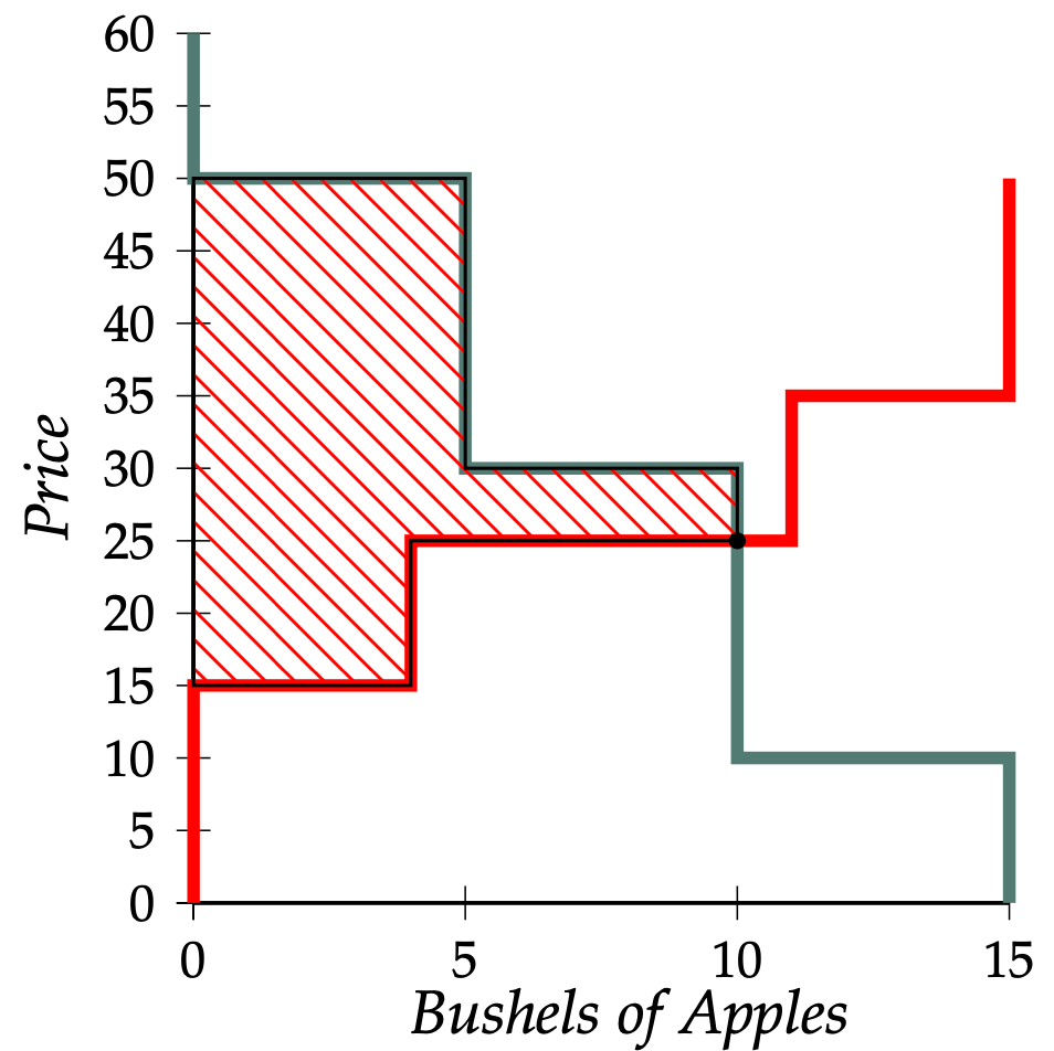
From Figure 1, we see that the competitive equilibrium price of apples is 25€ per bushel and the competitive equilibrium quantity sold is 10 bushels. As we discovered in Chapter 1, total profits made by buyers and sellers are equal to the shaded area between the demand curve and the supply curve to the left of the competitive equilibrium quantity. In this case, total profits made by buyers and sellers on apple transactions are 190€.2 But this is not the end of the story. Every bushel of apples that is produced imposes a cost of 1€ on everybody in the market (whether or not they made a purchase or a sale). Since 10 bushels are sold, this means that each of the 30 people in the market has to pay a pollution cost of 10€. Therefore the total cost of pollution to people in the market is 10€\(\times 30=\) 300€. When we subtract the 300€ in pollution costs from the 190€ in profits made on transactions, we find that the total amount of profit earned by people in this market is \(-\)110€! Remarkably, it turns out that total profits are lower when people are allowed to trade to a competitive equilibrium than they would be if there had been no trade at all.
How can it be that although everybody who trades makes a profit (or at least no loss) on the trade, total profits of all persons in the market are negative? The answer is that traders take account of their own costs, but do not account for the costs that they impose on others through negative externalities. Consider, for example, a supplier with Seller Cost 25€ who sells a bushel of apples to a buyer with Buyer Value 30€ for a price between 25€ and 30€. Both the buyer and the seller make a profit, and the total of the buyer’s profit and the seller’s profit is 5€. But producing this bushel of apples imposed a pollution cost of 1€ on each of the 30 people in the market. Although the buyer and seller together make a profit of 5€ on the transaction, they impose a negative externality of 30€, so that this sale reduced total profits in the market by 25€.
One might first think that since total profits are lower in competitive equilibrium than with no trade, the way to maximize total profits is to prohibit all trading in apples. But this turns out not to be the answer. To see why, consider a trade between a demander with Buyer Value 50€ and a supplier with Seller Cost 15€. Total gains of the seller and buyer from trading are 50€\(-\)15€\(=\)35€, and the total costs imposed by the externality are 30€. So this trade increases the total total amount of profits in the market by 35€\(-\)30€\(=\)5€.
In general, it may be economically efficient for the economy to allow some transactions, even if they impose negative externalities. The transactions that are consistent with efficiency are those in which the total profits to buyer and seller are greater than the total costs imposed by the associated externality. For such trades, the traders would still make a profit even if they had to compensate everyone in the market for the negative externality caused by their trade. On the other hand, trades in which the profits of buyer and seller are smaller than the total amount of externalities caused by these trades result in a reduction in total profits in the economy and are not economically efficient.
While trades between demanders with Buyer Values of 50€ and suppliers with Seller Costs of 15€ are economically efficient, you may well think that they are not fair. Why should individuals who make trades that impose negative externalities on others not have to pay their victims for damage done? Is it fair that trading between some individuals leaves others worse off than they would have been if no trades were allowed? We will demonstrate that with a pollution tax like the one in Session 2 of our experiment, it is possible to achieve efficiency while at the same time compensating those who are damaged by negative externalities.
We have seen that in a market with negative externalities and no controls on trader behavior, too many trades are made. One way to improve on this outcome is to introduce a pollution tax, just as we did in Session 2 of our experiment. In this session, sellers were taxed for each unit sold and all participants in the market received an equal share of the tax revenue. The effect of such a tax is that the supplier (at least partially) compensates everyone in the market for the pollution costs that her sales impose on others.
Suppose that the pollution tax on each sale is set equal to the total cost of the negative externalities that the sale imposes. Since the seller must pay the tax, she will be willing to sell a unit of output only if the price she is paid is at least as great as her Seller Cost plus the tax. Where the tax equals the total pollution costs imposed by producing one unit, she will sell only for a price that is greater than the sum of her production cost and the total pollution costs that she imposes by producing a unit. 3
In our previous example, the total cost of externalities generated in the production of a bushel of apples was 30€. Suppose that the government imposed a pollution tax of 30€, to be collected from the seller for each bushel of apples sold. The effect of this tax is the same as that of a 30€ increase in Seller Costs for all suppliers.4 The tax would therefore shift the supply curve vertically by 30€. This shifted supply curve is shown in Figure 2.
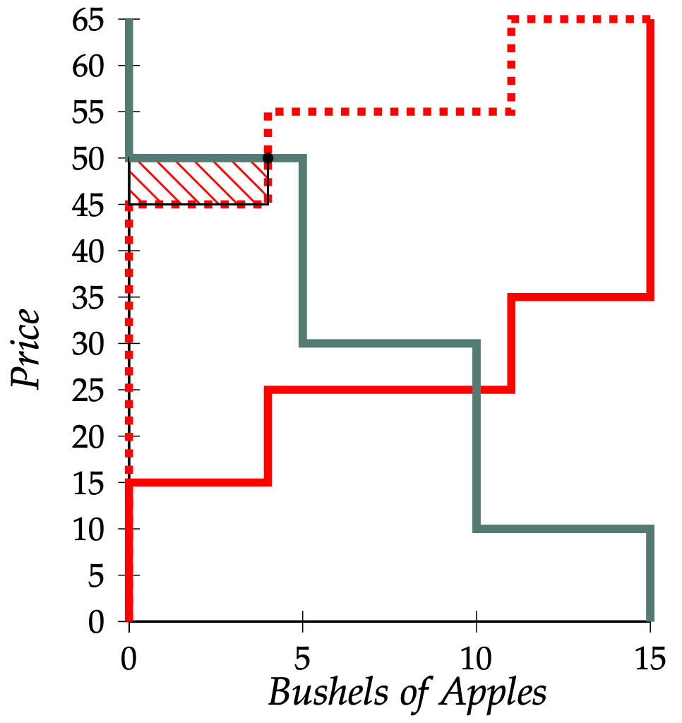
In Figure 2, we see that the shifted supply curve meets the demand curve where the price of apples is 50€ per bushel and the number of bushels sold is 4. These are the competitive equilibrium price and quantity with a 30€ pollution tax. Total profits made by buyers and sellers from apple transactions are given by the area between the shifted supply curve and the demand curve. These total profits are 5€\(\times 4=\) 20€. Since each unit sold is taxed at 30€, total tax revenue is 30€ \(\times 4 =\)120€. Since each of the 4 produced units causes 1€ worth of negative externalities to each of the 30 persons in the market, the total cost of externalities is 30€ \(\times 4 =\)120€. To find total profits in the market, we add buyers’ and sellers’ profits to the amount of tax revenue (which is returned to the market participants) and subtract the total externality costs. Thus we have total profits of 20€\(+\)120€\(-\)120€\(=\) 20€.
Let us see how these profits are distributed in the population. The only people who bought apples were four demanders who had Buyer Values of 50€ and who paid 50€ for a bushel of apples, so all of these buyers made zero profits. The only people who sold apples were four suppliers, who had Seller Costs of 15€, and who paid a tax of 30€. Since they received a price of 50€ for their apples and had costs of 15€\(+\)30€\(=\)45€, these sellers each made 5€ on the transaction. Every participant in the market suffered negative externalities of 4€ ( 1€ from each of the four bushels of apples produced), but everyone got an equal share of the tax revenue. Since there was 120€ in tax revenue to be divided among 30 people, each person received 4€ as their share of tax revenue; this exactly cancels the 4€ costs imposed on each person by the externality. When both the externalities and the divided tax revenue are taken into account, nobody is worse off than they would have been if production of apples had been prohibited, and the four sellers who sold apples are each better off by 5€.
In general, total profits in a market will be maximized if each individual takes into account the full externality costs of his or her actions. If a pollution tax on suppliers is set equal to the total cost of the externalities they impose, then the tax serves exactly this purpose. A supplier’s total costs will then include all of the costs that her activity imposes on society, the externalities that she generates as well as her own Seller Cost. In the apple market example, if apple producers must pay a 30€ tax, they will sell a bushel of apples only if they can get a price that is at least 30€ higher than their Seller Costs, which means that they will be able to make a sale only if the buyer’s Buyer Value exceeds the seller’s Seller Costs by at least the total cost of negative externalities imposed by the production of a bushel of apples.
In Session 3 of the experiment, we tried another method of controlling externalities. Each seller was required to have a pollution permit before being allowed to produce a unit of output. A fixed number of pollution permits was issued, and people were allowed to buy and sell these permits. Since suppliers must present a pollution permit for every unit of output that is produced, the total number of units produced cannot be greater than the number of permits issued.
Given the total number of permits, total profits made by buyers and sellers will depend on which suppliers are using the permits. If pollution permits were not marketable, the only suppliers who would be permitted to sell the good would be the ones who happened to own pollution tickets. If some high-cost suppliers had pollution tickets and some low-cost suppliers did not have pollution tickets, the outcome would be wasteful since output which could have been produced by low-cost suppliers would be produced by high-cost suppliers. If the government authorities know in advance which were the lowest-cost suppliers, they could achieve efficiency by awarding pollution permits only to the lowest-cost suppliers. But it is often difficult for policy-makers to determine who has the lowest costs. A simple way to ensure that pollution tickets will ultimately find their way into the hands of the lowest-cost producers is to allow the holders of pollution tickets to resell them.
To see that marketable permits will ultimately be used by the group of suppliers with lowest Seller Costs, let us consider an example. Suppose that the market price for apples is 50€ per bushel and suppose that Supplier \(A\), who has Seller Cost 35€, has a permit, while Supplier \(B\), who has Seller Cost 15€ does not. If Supplier \(A\) uses her permit to sell a bushel of apples for 50€, she will make a profit of 15€. Supplier \(B\) cannot make a sale unless she has a pollution permit, but if she had a permit, she could sell a bushel of apples for 50€, which is 35€ more than her Seller Cost. Therefore Supplier \(B\) would be willing to pay up to 35€ for a permit. Since \(A\) makes a profit of only 15€ from using the permit herself, it must be that both \(A\) and \(B\) could increase their profits if \(A\) sold her pollution permit to \(B\) for any price between 15€ and 35€. This reasoning leads us to expect that if suppliers are free to buy and sell pollution permits among themselves, the permits will eventually fall into the hands of those suppliers with the lowest Seller Costs.
The market for pollution permits will function much like the market for any other good. We should therefore be able to predict the equilibrium price of pollution permits using the tools of supply and demand. The “demanders” in the permit market are the suppliers of final goods, who need pollution permits in order to be allowed to produce. In Effluvia, the demanders for permits are the mine owners. In our apple market example, the demanders for permits are the suppliers of apples.
Regardless of the price of permits, the total supply of permits to the market is fixed at the number of permits issued by the government. This means that the supply curve for permits is a vertical line.
Plotting the demand curve for permits is a little more complicated. In the case of our apple market example, we need to figure out the amount that each apple supplier would be willing to pay for a pollution permit. This will depend on the number of permits issued. Suppose, that the government issues 4 pollution permits. Knowing this, everyone will realize that only 4 bushels of apples can be brought to market with pollution permits. Looking at the demand curve for apples in Figure 1, we see that if the supply of apples is 4 bushels, sellers would be able to sell their apples at a price of 50€ per bushel, but they could not sell any apples for a price higher than 50€. Given that they expect to be able to sell apples for 50€ a bushel, what would suppliers be willing to pay for a pollution permit?
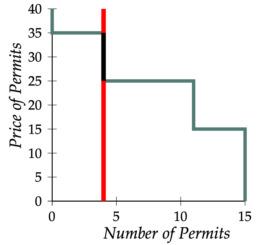
If she had a pollution permit, a supplier with Seller Cost 15€ could sell a bushel of apples for 50€ and would make a profit of 35€. Therefore she would be willing to pay up to 35€ for a pollution permit. With an apple price of 50€, a supplier with Seller Cost 25€ could make a profit of 25€ if she had a pollution permit, and hence would be willing to pay up to 25€ for a permit. By similar reasoning, a supplier with Seller Cost 35€ would be willing to pay up to 15€ for a pollution permit. Therefore the four suppliers with Seller Cost 15€ would be willing to pay 35€, the seven suppliers with Seller Cost 25€ would be willing to pay 25€, and the four suppliers with Seller Cost 35€ would be willing to pay 15€ for a pollution permit. These willingnesses-to-pay imply that the demand curve for pollution permits is as drawn in Figure 3.
Since the government makes exactly 4 pollution permits available, the supply curve for permits is a vertical line, corresponding to a fixed supply of 4 permits. From Figure 3, one can see that when 4 permits are available, the supply curve meets the demand curve along the line segment running from \((4,25)\) to \((4,35)\). This means that the market for pollution permits is in equilibrium at any price between 25€ and 35€ per permit.
In our analysis of the market for permits, we discovered that if four permits are issued, the competitive equilibrium price can be any price between 25€ and 35€. Let us have a look at supply and demand in the apple market if pollution permits sell for 30€. Since every supplier must have a pollution permit costing 30€ and must also pay her Seller Costs, the supply curve for apples is obtained by shifting the supply curve that applies when permits are not required upward by 30€. This shifted supply curve is shown as the dashed line in Figure 4.
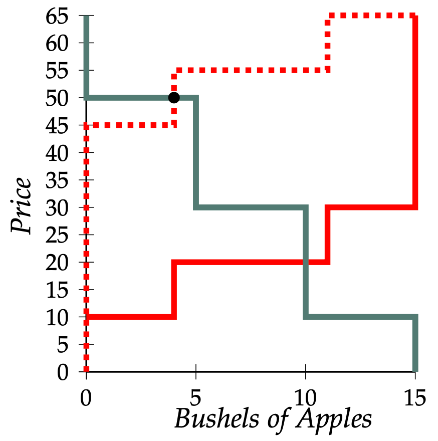
The requirement that suppliers must have permits does not affect buyers’ willingness-to-pay for apples, so the demand curve for apples remains unchanged. As we see from Figure 4, the demand for apples equals the supply of apples when the price is 50€ and the number of apples produced is 4 bushels. This is the same equilibrium that we found when we imposed a 30€ pollution tax.5
In order to achieve full efficiency, either with a pollution tax or with pollution permits, the government would need to have far more detailed information about supply, demand, and externalities than it is likely to be able to obtain. In order to set a pollution tax equal to the total cost of the negative externalities generated, the government would need precise information about these costs. In order to issue the right number of permits, the government would need to be able to calculate the economically efficient output in the polluting industry. While full efficiency may not be attainable with available information, it is likely that significant movements in the direction of efficiency can be made by using policies based on approximate information.
If the government knew the demand and supply curves perfectly, it would always be possible to attain the same goals of pollution reduction either by taxing pollution or by distributing a limited number of marketable pollution permits. But if the government is not sure about these curves, then it faces a choice between setting the tax at a certain level without knowing the resulting level of pollution, or of issuing a fixed number of pollution permits, so it knows the amount of pollution reduction in advance, but does not know the price of pollution tickets, and hence does not know in detail the effects on the price of goods produced. One of the benefits that governments have discovered when they issue marketable pollution permits is that they are able to observe the prices of these permits and thus make better estimates of the costs and benefits of changing air-quality standards.
Almost all of the pollution that an individual experiences is caused by others, rather than by himself or herself, so it is reasonable to make the simplifying assumption that buyers or sellers ignore the effect of their own trading on the total amount of pollution.↩︎
You can find this area by breaking up the shaded area into rectangles and adding the areas of these rectangles. One way to calculate this area is as follows: 35€\(\times 4+\)25€\(\times 1 +\)5€\(\times 5=\)190€.↩︎
A careful reader may notice that since 1/30 of the total amount of taxes collected will be rebated to each supplier, the true cost to a supplier of paying a 30€ tax is only 29€. The same careful reader might also notice that a clever supplier would be aware that her own production will cost her 1€ in pollution damage, and hence the profits that she gets from selling a unit are 1€ less than we have posited in drawing the supply and demand curves. It can be shown that these two effects exactly counterbalance each other, so that the outcome is precisely the same as if each supplier ignored the fact that she would share in the proceeds of the taxes that she paid and also ignored the cost to herself of her own pollution.↩︎
Taxes are studied in the Apple Market with a Tax Experiment.↩︎
If the price of pollution permits takes any other value in the equilibrium range, which runs from 25€ to 35€, the supply curve, which is shifted by the amount of the tax, will still intersect the demand curve at an output of 4 bushels of apples. Thus, all permit prices in the equilibrium range will result in the same efficient output of apples.↩︎