Version 1.01, October 2019
In this experiment you will learn that
when there are negative externalities, competitive trading can lead to inefficient outcomes;
it is not, in general, efficient to eliminate negative externalities entirely;
an appropriately chosen sales tax can improve efficiency when there are negative externalities; and
negative externalities can also be regulated in an efficient way by means of a fixed supply of marketable pollution permits.
To complete the exercises you need to know how to
shift supply and demand curves because of a per unit sales taxes.
Your instructor will provide LabNotes: the relevant information to study and interpret the results of the experiment. Use the data in the LabNotes to answer the questions in this section. The LabNotes will contain the following tables (identified by  ):
):
Transactions, prices, and profits in the last round of each session (tables \(A\)  , \(B\)
  , and \(C\)
Distribution of types (table \(D\)  ).
).
Pollution cost, amount of pollution tax in Session 2, and number of pollution permits in Session 3 (table \(E\)  ).
).
POLLUTION DAMAGES
Use Table \(E\)  to calculate the total cost of pollution in the last round of each Session of the experiment. In the first row enter the pollution cost that each resident of Effluvia suffers from a single unit of coal (table \(D\)
  ). In the second row record the number of units of coal traded (tables \(A\)
  -\(C\)
  ). In the third row calculate the total pollution cost suffer for each resident. In the fourth row record the total number of participants in the experiment, including any who did not buy or sell (table \(D\)
  ). Finally, compute the Total Cost of Pollution.
| Session 1 | Session 2 | Session 3 | |
| Per-Resident Damage by Each Unit of Coal | |||
| Units of Coal Burnt | |||
| Total Pollution Cost Per Resident | |||
| Number of Residents | |||
| Total Cost of Pollution |
EXPERIMENTAL OUTCOME
Complete Table 2 for the last round of Session 1 in your experiment using Table \(A\)  and Table \(E\)
  . Find total profits of all residents of Effluvia net of pollution costs, by subtracting the Total Cost of Pollution from the sum of the Profits of Sellers and Buyers from Transactions.
| Value | |
| Mean Price | |
| Units of Coal Sold | |
| Total Profits of Sellers from Transactions | |
| Total Profits of Buyers from Transactions | |
| Total Cost of Pollution | |
| Total Profits of All Residents | |
| Net of Pollution Costs |
Complete Table 3 for the last round of Session 2. Total tax revenue is equal to the units of coal sold time the pollution tax per unit. Add total after-tax profits of sellers, total profits of buyers, and total tax revenue, and then subtract the total cost of pollution to find total profits and tax revenue of all residents net of pollution costs in Effluvia.
| Value | |
| Mean Price | |
| Units of Coal Sold | |
| Total After-Tax Profits of Sellers from Transactions | |
| Profits of Buyers from Transactions | |
| Total Tax Revenue | |
| Total Cost of Pollution | |
| Total Profits and Tax Revenue of All | |
| Residents Net of Pollution Costs |
Compare total profits of all residents of Effluvia in Session 1 and Session 2. In which of the two sessions is total profits larger?
Complete Table 4 for the last round of Session 3. You can find the total revenue of permit sellers by summing the prices paid for permits as computed in Table \(C\)  . Add total profits of coal buyers, total profits of coal sellers, and total revenue of permit sellers, and then subtract the total cost of pollution, to get total profits of all residents net of pollution costs.
| Value | |
| Mean Price of a Unit of Coal | |
| Mean Price of a Permit | |
| Units of Coal Sold | |
| Total Profits of Sellers of Coal from Transactions | |
| Total Profits of Buyers of Coal from Transactions | |
| Total Revenue of Permit Sellers | |
| Total Cost of Pollution | |
| Total Profits of All Residents Net of Pollution Costs |
COMPETITIVE PREDICTIONS
Use the information in Table \(D\)  of your Lab Report to draw demand and supply curves in Figure 1 for the market in Session 1 where there is no governmental intervention. Mark the competitive equilibrium outcome and label it as CE1
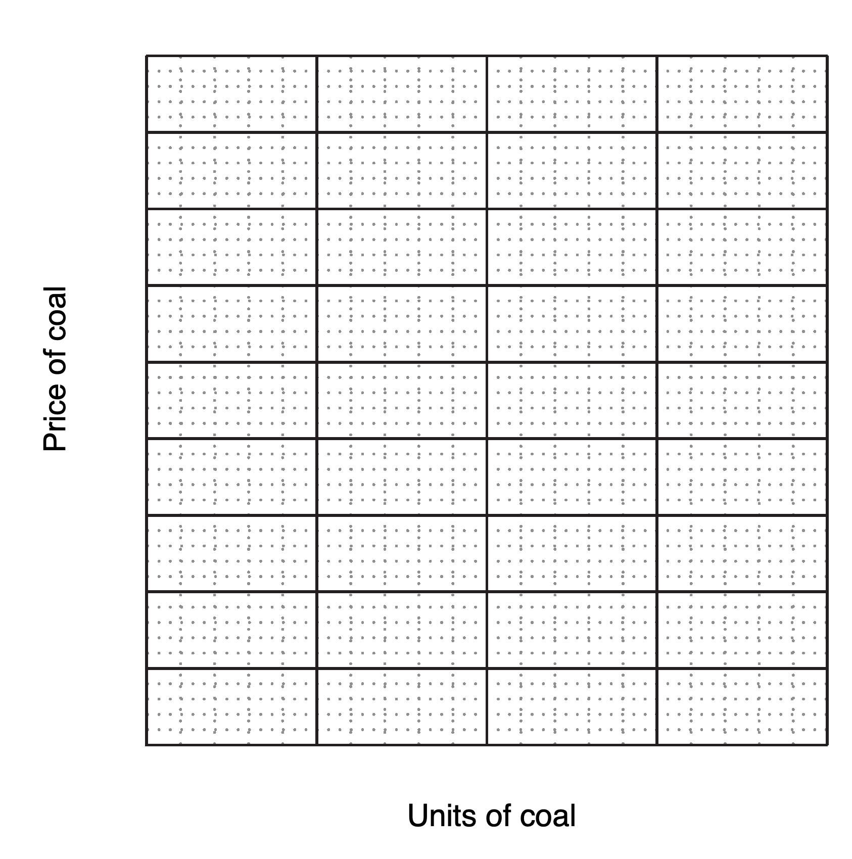
From the supply and demand curves that you drew in Figure 1, find the competitive equilibrium predictions and record them in Table 5.
| Value | |
| Price | |
| Units of Coal Sold | |
| Total Profits of Sellers from Transactions | |
| Total Profits of Buyers from Transactions | |
| Total Cost of Pollution | |
| Total Profits of All Residents Net of Pollution Costs |
In Session 2, the pollution tax is a sales tax collected from sellers. On Figure 1, use blue ink to draw the shifted supply curve after the pollution tax is introduced. Mark the competitive equilibrium outcome and label it as CE2.
From the supply and demand curves that you drew in Figure 1, find the competitive equilibrium predictions for Session 2 and record them in Table 6.
| Value | |
| Price | |
| Units of Coal Sold | |
| Total Profits of Sellers from Transactions | |
| Total Profits of Buyers from Transactions | |
| Total Tax Revenue | |
| Total Cost of Pollution | |
| Total Profits and Tax Revenue of All Residents, Net of Pollution Costs |
POLLUTION PERMITS
In Session 3, suppliers must have a permit in order to sell a unit of coal. Therefore, the units of coal supplied in Session 3 can be no larger than the number of permits issues, and the supply curve becomes vertical at that number. In Figure 1, draw a vertical supply curve for the quantity of permits issued. Use the demand curve to find the price at which the quantity demanded equals the number of pollution permits issued. This will be the equilibrium price of a unit of coal. What is the equilibrium prediction for the price of a unit of coal in Session 3?
In Table 7 copy the number of suppliers for each type from the data in your Lab Report. In the third column, enter the maximum amount that each type of supplier would be willing to pay for a pollution permit when the price of a unit of coal is the equilibrium price that you found in the previous question. (If there is a range of competitive equilibrium prices, assume that the price is at the midpoint of its range.)
| Seller Cost | Number in Market | Willingness to Pay for a Permit |
| 8 | ||
| 13 | ||
| 18 | ||
| 23 | ||
| 28 |
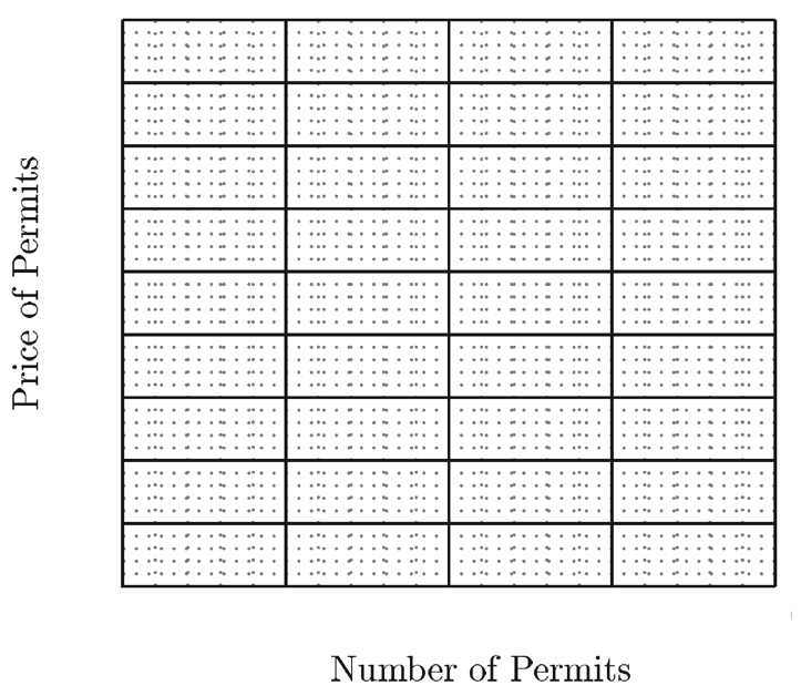
In Figure 2, use the information from Table 7 to draw the demand curve for pollution permits. On the same graph, draw a vertical supply curve at the number of permits that were issued in Session 3 of the experiment. The competitive equilibrium price for permits in Session 3 is:
