Version 1.01, October 2019
In this experiment, we apply supply and demand theory to explain the way that the price of fish and the revenue of fishermen respond to a change in the number of fish caught.1 Because of changes in the weather, fishermen caught many more fish in Session 2 than in Session 1. What prediction does competitive equilibrium theory make about the effect of a larger catch on the price of fish and on the profits of fishermen? We will answer this question by using a technique known to economists as comparative statics. Comparative statics is a tool for predicting the way that external causes such as the weather will affect economic variables. We will use this tool to study the effects of a change in the number of fish caught on market prices, on profits, and on consumers’ surplus.
The recipe for comparative statics analysis is simple. First draw the supply and demand curves that apply before the change and look at the predicted equilibrium values of the economic variables of interest. Then draw the supply and demand curves that apply after the change and predict the new equilibrium values. Finally, compare the equilibrium values of these variables before and after the change.
The key to comparative statics analysis is to answer two questions: “What happened to the supply curve?” and “What happened to the demand curve?” Let us apply these two questions to the fish-market experiment.
Recall that the supply curve shows the number of fish that fishermen would be willing to sell at any possible price. In this experiment, the fishermen’s only costs are for the fuel they purchased the night before. These costs are known as sunk costs, since fishermen must pay them even if they don’t sell any fish.2 As you found in the warm-up exercises, fishermen are better off accepting any positive price for their fish rather than leaving the fish to rot on the beach.
So what does the supply curve for fish look like? At any positive price, every fisherman will want to sell all of his fish. Therefore the supply curve includes a vertical line segment that meets the horizontal axis at the total number of fish caught by fishermen. This vertical line is shown as the dashed line in Figure 1 for a case where 15 fish are caught. At a price of zero, fishermen will be just indifferent between selling their fish or not, so the supply curve also includes a horizontal segment running from the origin to the point on the horizontal axis where the vertical segment begins. In Figure 1, this is the line segment extending from the origin to the point \((15,0)\).
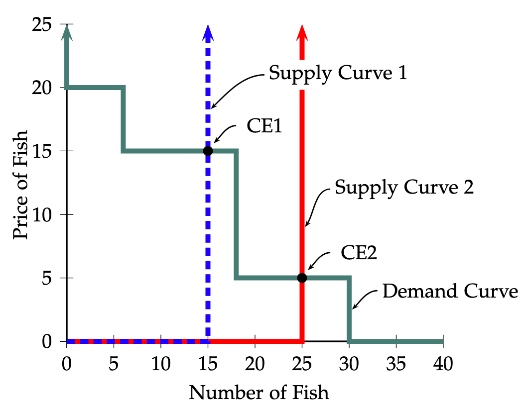
In Session 2 of our experiment, the total number of fish caught is different from that in Session 1, but fishermen will again want to sell all of their fish at any positive price. Therefore the new supply curve includes a vertical line segment that meets the horizontal axis at the number of fish caught in the second session, and a horizontal line segment extending from the origin to the bottom of the vertical segment. For example, if the new number of fish caught happened to be 25, then the supply curve would be as shown by Supply Curve 2. The vertical segment meets the horizontal axis at \((25,0)\) and the horizontal segment extends from the origin to \((25,0)\). The effect of the change in the size of the catch was to shift the vertical portion of the supply curve for fish outward by the number of additional fish caught.
In this experiment, although the number of fish caught in the two sessions differed, the number of demanders did not change, nor did the distribution of demanders’ Buyer Values. This means that at any given price, the total number of fish demanded is the same in the two sessions. Therefore the demand curve did not change at all.
Let’s work through a complete comparative statics exercise for the case depicted in Figure 1. Suppose that on Day 1 the total number of fish caught was 15, and on Day 2 the total number caught was 25. On Figure 1, the supply curve for Day 1 is given by the dashed line labeled Supply Curve 1 and the supply curve for Day 2 is given by the solid line labeled Supply Curve 2.
The demand curve remains the same on both days. We see that competitive equilibrium on Day 1 is at the point \(CE1\) and competitive equilibrium on Day 2 is at the point \(CE2\). Thus when the number of fish caught increases from 15 to 25, the price of fish falls from 15€ to 5€ per fish, and total revenue of fishermen falls from 15€\(\times 15=\)225€ to 5€\(\times 25=\)125€.
An article in the August, 2019 edition of Outdoor News, reads :
Salmon prices falling in wake of California fishing boom. “Commercial salmon catches have surpassed official preseason forecasts by about 50%, \(\dots\) This year’s adult salmon are the first class to benefit from record rainfall that filled California rivers and streams in early 2017, making it easier for juvenile chinook to migrate to the Pacific Ocean, where they grow into full-size fish. \(\dots\) For consumers, the bountiful harvest has driven down wild salmon prices to 15€ to 20€ per pound, compared with 30€ to 35€ per pound in recent years. Fishermen are making up for the difference by catching more fish. ”
A story in the Wall Street Journal, a few years earlier reported:
Fishermen in Alaska, Awash in Salmon, Strive to Stay Afloat. ‘Alaska is awash in salmon. Huge fish runs have been building here. Combined with the growing output from sources like Chilean fish farms and Russian fishing fleets, they are glutting the market and driving wholesale prices to record lows.’’
The story goes on to say that the price of salmon has fallen to five cents a pound from a peak price of eighty cents a pound eight years ago. It quotes a fisherman who
“figures he would have to catch nearly a million pounds of salmon this summer to cover his boat payment and expenses for his three-man crew. \(\dots\) Its a weird problem. You love to catch fish, but the more you catch the less they’re worth.”
Stories like this are not rare. If you follow the business pages of any major newspaper, in almost any week you will find a report on how external events such as changes in the weather have changed the size of harvests in agriculture or fisheries, and how commodity prices respond to these changes.
The United States Department of Agriculture (USDA) issues monthly estimates of the size of agricultural crops. These estimates are almost always followed by news stories about their effects on prices. A July, 2019 article in the Wall Street Journal reads:
Corn prices soar as U.S.D.A. slashes crop forecast “\(\dots\)the U.S. Agriculture Department cut its estimates for global harvests of key crops and raised some demand forecasts \(\dots\) With yesterday’s gains, prices of corn futures contracts are now up 94% from their June lows; soybeans are up 51% and wheat is up 80% \(\dots\) The USDA’s revisions reflect the impact of dry weather in South America and floods in Australia, which have compounded supply constraints that first started to emerge in the middle of last year, when a drought in Russia ravaged that country’s wheat fields. The agency also cut estimates for U.S. harvests of corn and soybeans.
In June, 2019, the US Department of Agriculture forecast the size of the corn crop to be about 5% smaller than the previous year’s crop. The price of corn was 4.50€ per bushel as compared to 3.80€ a year earlier. In August, 2019, the USDA revised its forecasts sharply upward, reporting that farmers had planted more corn than expected and that good weather was producing healthy crops. The size of the total crop was now predicted to be similar to that in 2018. At this announcement, corn prices per bushel fell about 4.50€ per bushel to about 3.90€.
Industries like agriculture and fishing are vulnerable to unexpected shifts in total supply, which can dramatically change the price of their output. Farmers face much the same problem that our fishermen did. Most of their expenses are incurred in the spring, when they prepare the soil and plant and fertilize their crops. Returns on this investment do not come until fall when they harvest their crops. When they plant, they do not know how large their own harvests will be, nor do they know the price at which they can sell their product. This depends on unforeseeable events, like the weather.
When autumn comes, if the price of corn is low, farmers cannot get their expenses back by unplanting their corn. Their only options are to harvest their crops and sell for the going price or to leave them in the fields. As long as the price is higher than the cost of harvesting, farmers will want to sell their crops. The cost of harvesting is a small fraction of the total cost of producing a crop of corn. There are many years in which the price of a bushel of corn is high enough so that it is worthwhile for farmers to harvest the crop, but not high enough to repay all of the money that they have invested in it. In these years, farmers will harvest and sell the crop for whatever it brings, despite the fact that they have lost money. They may wish that they hadn’t planted corn in the spring, but it is too late to undo that decision. These farmers, like the fishermen in our experiment, cannot hope to recover their entire initial investment. The best that they can do to minimize their losses is to sell their output at the going price.
Costs that are already incurred and cannot be reduced by altering production are known as sunk costs or fixed costs. Costs that vary with the number of units sold are called variable costs. In the instance of the corn farmer, at harvest time the costs of planting the corn, caring for it, and fertilizing it are sunk costs. At this time, the only variable cost is the cost of harvesting, which could be avoided by leaving the crop in the fields. The decisions of farmers to harvest and sell crops that they have already planted, like the decisions of fishermen to sell fish that they hare already caught, are known as short-run decisions.
Economists also study long-run decisions, by which we mean forward-looking decisions taken at a time when sunk costs are not yet sunk. For the fishermen of our experiment, in the morning when they come in with their fish, the cost of last night’s fuel is a sunk cost. But in the afternoon, before fishermen refuel their boats, they may be able to decide whether or not to go fishing at all. At this time, their fuel costs are variable costs. When they make the decision of whether or not to go fishing, the fishermen can avoid fuel costs by leaving their boats in the harbor. Of course, if they do so they will catch no fish. For farmers, the cost of planting is a fixed cost at harvest time, but it is a variable cost in the spring. If the farmer chooses not to plant any crops he can avoid all of these costs. Of course, if he does so he will have no crops to sell in the fall.
Since weather conditions, the size of the harvests, and the price of output are unpredictable, we can expect there will be times when fishermen and farmers do not recover their sunk costs and also times when they get back more than they have spent. If on average, over the years, fishermen or farmers do not recover their sunk costs, then at least some of them will go out of business. Perhaps you can guess what the effects of this will be. A reduction in the number of fishermen or farmers will reduce the amount of product supplied at any price, thus shifting the supply curve to the left and causing the price to be higher in future periods.
It turns out that the principles that we have discussed for fishing and agriculture apply in much the same way to many other industries, including manufacturing and service industries. You will study these principles in more detail if you participate in the Restaurant Market Experiment, where we deal with short-run and long-run decision-making in the restaurant business.
Click the links if you need to learn how to draw supply [here] and demand [here] curves or to find competitive equilibrium prices and quantities [here].↩︎
If you participated in the Apple Market Experiment, you may remember that, in contrast, suppliers had to pay their Seller Cost only if they sold a bushel of apples. They did not have to pay this cost if they did not sell.↩︎