Version 1.01, October 2019
In this experiment you will
Become acquainted with the mechanics of a simple trading-pit environment.
Learn to apply the concepts of competitive supply and demand to a very simple market.
Learn to draw supply and demand curves corresponding to given market data, and to read market data from given supply and demand curves.
Learn to compare results in an experimental market with the theoretical predictions of the competitive model.
Begin to understand the benefit of having an abstract theory for predicting the effects of changes in the environment.
Learn to test a proposed theory by confronting it with experimental data.
Learn to calculate consumer surplus, seller profits and total surplus.
Your instructor will provide LabNotes: the relevant information to study and interpret the results of the experiment. Use the data in the LabNotes to answer the questions in this section. The LabNotes will contain the following tables (identified by  ):
):
Transactions, prices, and profits in the last round of each session (tables \(A\)  and \(B\)
  ).
).
Distribution of types in each Session (tables \(C\)  and \(D\)
  ).
).
Use the information in tables tables \(A\)  and \(B\)
  to complete Table 1. Count the number of transactions recorded in each session and find the mean (average) price by adding all the prices posted and dividing by the number of transactions. Find total profits of sellers and of buyers by adding the corresponding columns in these tables. Find total profits of all traders by adding total profits of sellers and total profits of buyers.
| Session 1 | Session 2 | |
| Mean Price | ||
| Number of Transactions | ||
| Total Profits of Sellers | ||
| Total Profits of Demanders | ||
| Total Profits All Participants |
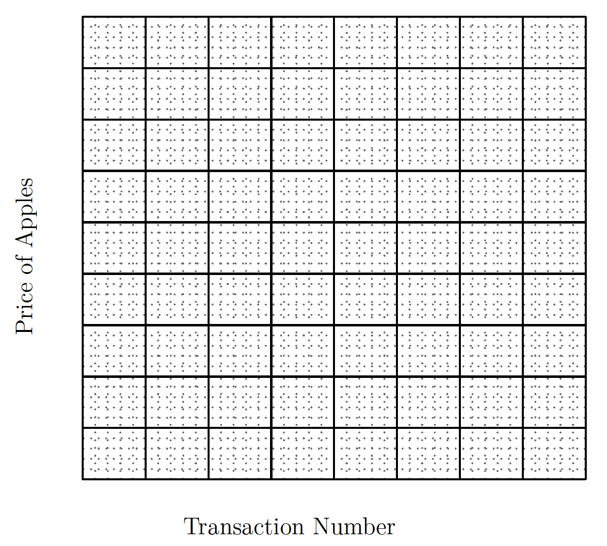
When you are looking for logical patterns in a mass of numerical information, it is often useful to draw a graph. One way to present the results of this experiment is to plot a time series of prices, showing the transaction prices in the order in which they were recorded. In Figure 1, plot the time series of prices in the last round of Session 1 in red ink and the time series of prices in the last round of Session 2 in blue ink. To plot these paths, use the numbers entered in Tables \(A\)  and \(B\)
  . To plot the time series of prices, mark the point \((1,P_1),(2,P_2)\), and so on, where \(P_1,P_2,\dots\) are the prices in the first, second, \(\dots\) transactions. Finally, draw line segments that “connect the dots” that you have plotted.

Complete the Supply and Demand Tables 2, 3, 4, and 5 for Sessions 1 and 2. These tables will be used to draw supply and demand curves for each session. The information needed to complete these tables is found in tables \(C\)  and \(D\)
  . [Click here and here if you need help on how to construct supply and demand tables, respectively.]
| Price Range | Amount Supplied |
| \(P <\) 10€ | |
| 10€ \(< P<\) 30€ | |
| \(P>\) 30€ |
| Price Range | Amount Demanded |
| \(P>\) 40€ | |
| 20€ \(< P <\) 40€ | |
| \(P<\) 20€ |
| Price Range | Amount Supplied |
| \(P<\) 10€ | |
| 10€ \(< P<\) 30€ | |
| \(P>\) 30€ |
| Price Range | Amount Demanded |
| \(P>\) 40€ | |
| 20€ \(< P<\) 40€ | |
| \(P<\) 20€ |
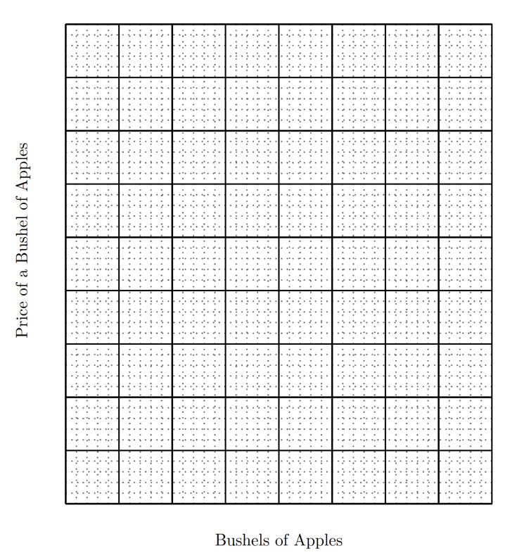
In Figure 2, use the information from the Supply and Demand Tables 2 and 3 to draw a (red) supply curve and a (green) demand curve for the market in Session 1. Mark the intersection of the supply and demand curves with a black dot and label it \(CE\). [Click here. if you need help on how to draw a supply curve; or click here if you need help on how to draw a demand curve.]

In Figure 3, use the information from the Supply and Demand Tables 4 and 5 to draw a (red) supply curve and a (green) demand curve for the market in Session 2. Mark the intersection of the supply and demand curves with a black dot and label it \(CE\).

Complete Tables 6 and 7 to compare the experimental results from your classroom experiment with the predictions made by supply and demand theory. Hints: \(\bullet\) The predictions of the theory and the actual outcomes of the experiment are two different things. The information about experimental outcomes can be copied from Table 1. The predictions of the theory can be obtained from the competitive equilibrium in figures 2 and 3. [Click here if you need help with finding the equilibrium; or here if you need help on computing consumer surplus and seller profits.] \(\bullet\) Market efficiency of an experimental outcome is defined as the actual total profits of as percentage of the highest possible amount of profits that could be achieved in the market. The competitive prediction of market efficiency is 100 percent, meaning that the highest total amount of profit for a market like the one in this experiment is achieved in competitive equilibrium. This tells you that the efficiency of your experimental outcome can be obtained by expressing total profits of all traders in the market experiment as a percentage of the predicted total profits in competitive equilibrium.
| Experimental Outcome | Competitive Prediction | |
| Mean Price | ||
| Number of Transactions | ||
| Total Profits of All Sellers | ||
| Total Profits of All Buyers | ||
| Total Profits of All Traders | ||
| Market Efficiency | 100% |
| Experimental Outcome | Competitive Prediction | |
| Mean Price | ||
| Number of Transactions | ||
| Total Profits of All Sellers | ||
| Total Profits of All Buyers | ||
| Total Profits of All Traders | ||
| Market Efficiency | 100% |
Not only does competitive equilibrium theory predict prices, quantities, and profits, it also makes predictions about which traders will trade and which will not. Complete Tables 8 and 9 to compare the experimental outcomes with competitive predictions. Hint: You can determine the number of persons of each type who actually traded by looking at the transaction tables in your Lab Notes. The number of persons of each type who trade in competitive equilibrium can be obtained from figures 2 and 3. Recall that the demand curve lines up demanders according to their Buyer Value, from the highest to the lowest. Similarly, the supply curve lines up suppliers from the lowest seller cost to the highest.
| Experimental Outcome | Competitive Prediction | |
| Number of Low-Cost Sellers | ||
| Number of High-Cost Sellers | ||
| Number of High-Value Buyers | ||
| Number of Low-Value Buyers |
| Experimental Outcome | Competitive Prediction | |
| Number of Low-Cost Sellers | ||
| Number of High-Cost Sellers | ||
| Number of High-Value Buyers | ||
| Number of Low-Value Buyers |
Consider a market in which the distributions of Buyer Values and Seller Costs are as recorded in Table \(C\)  . Suppose that you are appointed as a middleman for the market. As the middleman, you can arrange the market by assigning trading partners–one supplier to one demander. Suppliers and demanders are not allowed to trade with anybody except the trading partner that you assign to them.
Suppose that you receive a commission of 1€ from the buyer and 1€ from the seller for every trade that takes place. If a pair of trading partners that you have assigned can both make a profit after paying your commission, they will trade. If they cannot both make a profit after paying your commission, they will not trade. You always choose to assign trading partners in such a way as to maximize your total income from commissions. What is the largest number of mutually profitable trades that you can arrange, and how much income in commissions will you make? Compare total profits of buyers and sellers plus the total revenue from your commissions with the total profits from all traders that you obtained in the competitive prediction (Table 6).
Hint: Try matching high-cost suppliers with high-value demanders and letting them trade at higher prices than the prices at which low-cost suppliers trade with low-value demanders.
Suppose that for the market in the previous problem, you are again a middleman, but instead of getting a commission of a fixed amount of money per transaction, you get to keep all of the profits of buyers and sellers. How would you arrange transactions so as to maximize your own profits?
Suppose that for the market in the previous problem, you are a middleman who is paid a certain fraction, say 10%, of the total profits of buyers and sellers. How would you arrange transactions so as to maximize your own profits?
Suppose that the distributions of Buyer Values and Seller Costs are as recorded in Table \(C\)  and that there is a legal requirement that every trade between a buyer and a seller must split total profits from the trade equally between the buyer and the seller. Buyers and sellers can meet and bargain as in our experimental sessions. A trade will occur only when a buyer and a seller agree to trade with each other and split the profits.
In equilibrium, who would trade with whom and at what prices would they trade?
Compare the number of trades and total profits from this outcome with the number of trades and total profits in competitive equilibrium.
Which traders are better off than they would be in competitive equilibrium? Which traders are worse off?