Version 1.01, October 2019
An excise tax is a tax placed on a specific good or services, such as gasoline,1 cigarettes,2 marijuana,3 airline tickets, or alcohol. An excise tax is sometimes called a "sales tax”, but the term sales tax is more commonly used to describe a broad-based tax assessed on almost all consumer goods at a fixed percentage of price. This discussion concerns the effect of excise taxes.4
When you fill up your tank at the gas pump, the meter shows the total price per gallon that you must pay. The amount of gasoline sold is reported to the government and the station owner is assessed taxes of a fixed amount per unit of gasoline sold. Excise taxes are usually collected from the sellers rather than the buyers, probably because sellers are easier to keep track of.5
If the government puts an excise tax on beer, soft drinks, cigarettes, hotel rooms, or luxury yachts, who pays the cost of the tax? When an excise tax is proposed for some good, there are usually loud complaints from sellers, who believe that the tax will come out of their profits, and from buyers, who think that the entire tax will be passed on to them in the form of higher prices. Who is right?
At first glance, it seems plausible that since the seller has to pay the excise tax, the seller must bear all or most of the burden of the tax in the form of reduced profits. On the other hand, our classroom experimental results indicate that, at least for the specific distribution of Seller Costs and Buyer Values used there, a tax paid by the suppliers is partially passed on to buyers through higher prices. We also saw that when the buyers have to pay the tax, the tax burden is shared with the suppliers, who now receive lower prices. In fact, the after tax cost to buyers and the after-tax payment to sellers appear to be about the same, whether the tax is collected from buyers or from seller.
Competitive equilibrium theory gives us a powerful tool to study the effects of an excise tax. The key is to look at how the tax affects the supply and demand curves for the taxed good, and then consider the effect on equilibrium.
It is helpful here to introduce a bit of new notation. Let \(p_D\) be the cost to a demander of a unit of the good, including any taxes that demanders must pay. Let \(p_S\) be the net amount that suppliers receive per unit sold, net of any taxes they have to pay. The quantity demanded at price \(p_D\) is given by a function \(D(p_D)\) and the quantity supplied at price \(p_S\) is given by a function \(S(p_S)\). Supply equals demand when
\[\label{SequalD} D(p_D)=S(p_S).\qquad (1)\]
When the suppliers have to pay the tax, for each unit they sell they get a payment of \(p_D\) from demanders, but they have to pay a tax of \(t\), so their net receipt is
\[\label{suppay} p_S=p_D-t.\qquad (2)\]
We can find the equilibrium outcome, by solving the two equations (1) and (2) for the two unknowns \(p_D\) and \(p_S\).
When the demanders have to pay the tax, for each unit they buy, they pay an amount \(p_S\) to the suppliers, and they also have to pay a tax of \(t\), so the total amount they must pay is
\[\label{depay} p_D=p_S+t.\qquad (3)\]
Therefore when demanders pay the tax, equilibrium is found by solving the two equations (1) and (3) for \(p_D\) and \(p_S\).
But it is easy to see that Equation (3) is equivalent to Equation (2) . Therefore the equilibrium solutions for \(p_D\) and \(p_S\) are the same whether the tax is collected from demanders or from suppliers.
Thus we have the following general result.
Proposition: The competitive equilibrium after-tax price paid by buyers (\(p_D\)) and the after-tax price paid to sellers (\(p_S\)) are the same, whether the tax is collected from sellers or from buyers.
It follows that the equilibrium quantity is not affected either by who collects the tax. And, therefore, consumer surplus and buyer profits are also the same in both cases. These results allow policymakers to use other criteria, instead of tax incidence, when deciding on whom to impose a tax, like political feasibility or efficiency in collecting and monitoring. Just imagine you had to keep all your receipts for every drink, meal, movie ticket, grocery,... you buy and file taxes every four months; or the daunting task of the government to make sure you do not miss any of those tickets. As another example, it is easier to convince voters of supporting a pollution tax on the polluting firms than on the consumers of the product.
We begin with three examples. In Example 1, the burden of the tax is shared about equally between buyers and sellers. In this example, when a tax is collected from sellers, the equilibrium after-tax price paid by buyers rises by about half of the amount of the tax, so that the seller’s net revenue per sale decreases by about half of the tax.
In Example 2, with a horizontal supply curve, the equilibrium price paid by buyers rises by the full amount of the tax, so that the entire burden of the tax falls on demanders. In Example 3, with a vertical supply curve, the equilibrium price paid by buyers remains unchanged, so that suppliers’ after tax revenue per sale falls by the entire amount of the tax.
Let us illustrate the effects of an excise tax collected from suppliers, using supply and demand curves. Suppose that the distributions of seller costs and buyer values are as in the table below.
| Seller’s Costs | Number in Market | Buyer’s Value | Number in Market |
| 3 | 2 | 45 | 2 |
| 8 | 2 | 40 | 2 |
| 13 | 2 | 35 | 2 |
| 18 | 2 | 30 | 2 |
| 23 | 2 | 25 | 2 |
| 28 | 2 | 20 | 2 |
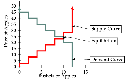
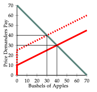
The corresponding supply and demand curves are shown in Figure 1.6 Notice that the supply and demand curves in Figure 1 do not cross each other at just a single point, but meet and run together along the interval from \((10,23)\) to \((10,25)\), where the number of trades is 10 and the price can be anything between 23€ and 25€. Thus the competitive model predicts that 10 bushels of apples will be sold. Instead of predicting a unique equilibrium price, the theory says only that the price will lie somewhere in the interval from 23€ to 25€.
Now suppose that a 15€ per-unit excise tax is charged to sellers. Let us draw supply and demand curves with the price that demanders pay to suppliers shown on the vertical axis. How does the tax affect the supply curve? Any supplier who sells a bushel of apples now has to pay a 15€ tax in addition to her production cost. Therefore the tax has the same effect on the supply curve as would a 15€ increase in Seller Costs for each supplier. This means that each point on the supply curve must be drawn 15€ higher than it was on the original supply curve. Economists describe this change by saying that the tax "shifted the supply curve upward” by 15€. Figure 2 shows the pre-tax supply curve as a solid line and the post-tax supply curve as a dashed line.
How does this sales tax affect the demand curve? That’s easy. Since Buyer Values do not change and buyers do not have to pay any tax, the tax does not change any demander’s willingness-to-pay (reservation price) for apples. Therefore the demand curve will be the same as it was without taxes.
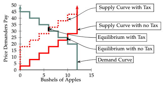
Looking at the supply and demand curves in Figure 2, we can find the effect of the tax on competitive equilibrium prices and quantities. The equilibrium without a tax is indicated by the darkened interval marked "Equilibrium with no Tax.” Without a sales tax, 10 bushels are sold and the price must be in the interval between 23€ to 25€. The competitive equilibrium with the tax is marked by the darkened interval marked "Equilibrium with Tax,” where the dashed supply curve meets the demand curve. On this interval, 6 bushels of apples are sold and the price must be somewhere in the interval between 30€ to 33€.
We see that the sales tax, when collected from sellers, decreases the number of trades from 10 to 6 and causes the price that consumers must pay to rise from somewhere in the interval between 23€ and 25€ to somewhere in the interval between 30€ and 33€. Thus buyers pay, on average, 7€ or 8€ more per unit than without the tax. Without the tax, sellers are paid somewhere between 23€ and 25€ per unit. In equilibrium with the tax, the price has risen by 7€ or 8€, but they have to pay a tax of 15€ per unit, so their payment net of taxes falls by 7€ or 8€.
In this example, the distribution of Buyer Values and hence the demand curve are the same as in Example 1. But this time we assume that there is a large number of potential suppliers, each of whom has a seller cost of 23€, and there are no suppliers with lower costs. When this is the case, the supply will be zero at any price below 23€ and at a price of 23€, many suppliers are willing to sell a unit. Thus the demand curve when there is no tax is as shown by the solid red lines in Figure 3.
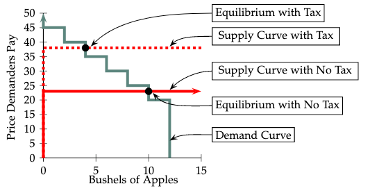
If a tax of 15€ per bushel of apples is collected from sellers, then the cost of supplying a bushel of apples rises from 23€ to 38€. No supplier would be willing to sell apples at a price below 38€ per bushel. At a price of 38€ per bushel supply becomes available from many suppliers. With the tax, the supply curve becomes the red dashed line in Figure 3
Figure 3 shows that without the tax, there is a competitive equilibrium in which the price is 23€ per bushel and 10 bushels are sold. With the tax, the equilibrium price rises to 38€ and only 4 bushels are sold. In this case, we see that in equilibrium, the entire amount of the tax is passed on to demanders. Demanders pay a price that is 15€ higher than it would be without the tax, and suppliers get the same after price revenue per unit with or without the tax.
In this example, the demand curve remains as in Examples 1 and 2. The supply curve however is horizontal in the relevant region. There are 10 suppliers, each of whom has seller costs of 1€ per bushel of apples. Each of the 10 suppliers will be willing to sell one bushel of apples for any price of 1€ or more. At prices below 1€, no apples would be sold. Therefore the supply curve when there is no tax is shown by the red line segments in Figure 4.
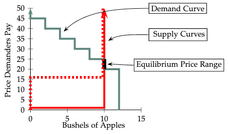
When the suppliers have to pay a 15€ excise tax for each bushel of apples sold, they will supply no apples at prices below 16€, their seller cost plus the tax. At prices of 16€ or higher, each of the 10 suppliers is willing to sell a bushel of apples, so the supply is 10. The supply curve with the tax is shown by the dotted line in Figure 4. We see that at all prices above 15€, the supply curve with the tax is the same as the supply curve without the tax. As the figure shows, the number of bushels sold and the competitive equilibrium price paid by demanders is the same with the tax as without the tax. This means that in this case, the suppliers can pass none of the tax burden on to the demanders. In equilibrium, the tax costs the demanders nothing, but reduces the profits of suppliers by 15€ per bushel sold.
As Examples 1-3 demonstrate, a tax that is collected from suppliers may be partially passed on to demanders, totally passed on to demanders, or not passed on at all. In general, the fraction of a tax that is passed on from suppliers to demanders in equilibrium depends on the "relative steepness” of the supply and demand curves.
Let us consider two more examples. In these examples the supply and demand curves are straight line segments.7 The green line is the demand curve, the solid red line is the demand curve with no tax, and the dashed red line is the supply curve when suppliers must pay a tax of 15€ per bushel.
In Figure 5, the slope of the demand curve is \(-1\) and that of the supply curve is \(+1/2\). With no tax, there is a competitive equilibrium with 40 bushels of apples sold at a price of 30. With the 15€ tax, the equilibrium price paid by demanders increases by 10€ from 30€ to 40€ and the the after-tax payment that suppliers receive per bushel falls by 5€ from 30€ to 40€\(-\) 15€\(=\) 25€. The quantity of apples sold falls from 40 bushels to 30 bushels. In this example, suppliers are able to pass 10€ of the 15€ tax on to the demanders in the form of higher prices.
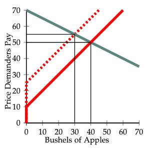
In Figure 6, the slope of the demand curve is \(-1/2\), and that of the supply curve is \(+1\). In equilibrium without a tax, 40 apples are sold at a price of 50€. In equilibrium with the tax, demanders pay 55€ per bushel and suppliers receive after-tax revenue of 40€ per bushel. Thus, only 5€ of a 15€ tax collected from suppliers is passed on to demanders.
In the market of Figure 5, the the "burden” of the 15€ tax is split, with a price increase to demanders of 10€ per bushel and a reduction of 5€ per unit in after-tax payments to suppliers. In the market of Figure 6, a 15€ tax results in a price increase of 5€ for demanders and reduction of 10€ per unit in after-tax payments for suppliers.
In Figure 5, the demand curve with slope \(-1\) is twice as steep8 as the supply curve with slope \(1/2\), and the demanders bear twice as large a share of the cost of the tax as suppliers. In Figure 6, the demand curve, with slope \(-1/2\) is only half as steep as the supply curve and suppliers bear twice as large a share of the cost as demanders.
This result generalizes as follows:
Proposition The ratio of the tax burden borne by demanders to that borne by suppliers is equal to the ratio of the steepness of the demand curve to that of the supply curve.
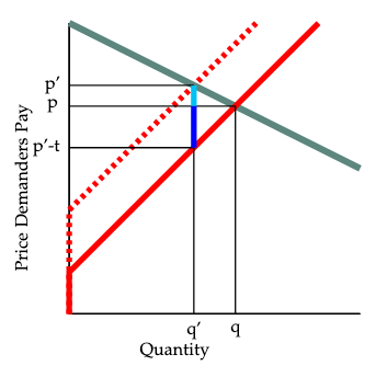
We sketch a proof of this proposition, using Figure 7. With no tax, the equilibrium quantity \(q\) and price \(p\) are found where the solid red supply curve crosses the demand curve. With a tax of \(t\) per unit collected from suppliers, the supply curve shifts upward by \(t\) units, and the equilibrium quantity falls from \(q\) to \(q'\). When the tax is imposed, the increase in the price paid by demanders is determined by moving up the demand curve as the quantity falls from \(q\) to \(q'\). This change is shown by the light blue line segment. When the quantity falls from \(q\) to \(q'\), the after-tax price received by suppliers is found by moving down the red supply curve. This change is shown by the dark blue line segment. Since the change in equilibrium quantity is the same for buyers and sellers, the ratio of the absolute value of the change in price paid by demanders to that of the after-tax price received by sellers must be equal to the ratio of the slope of the demand curve to the slope of the supply curve.9
If you have studied the concept of elasticity, you’ll know that economists like to describe the responsiveness of quantities demanded and supplied to price by the elasticity of demand and elasticity of supply.10 Since we show supply and demand with quantity on the horizontal axis and price on the vertical axis, the supply or demand curve is steeper if quantity is less responsive quantity is to price. In the extreme case where a demand or supply curve is vertical, we say that demand or supply is perfectly inelastic. Where a demand or supply curve is horizontal, we say that demand or supply is perfectly elastic.
If the demand curve is less steep than the demand curve, we say that demand is more elastic than supply. If the supply curve is less steep than the demand curve, we say that supply is more elastic than supply. For tax incidence, it helps to think of the elasticity as the flexibility or capacity to avoid the burden of the tax. Therefore, our tax incidence result says that the less elastic group (buyers or sellers) will bear a higher share of the tax, since they are more "rigid" in adapting their quantity to changes in the price. In the extreme case of, for example, a perfectly inelastic demand, consumers always buy the same quantity, independent of the price, and suppliers are able to shift the whole burden of the tax to them through a higher price.
An excise tax typically reduces profits of both suppliers and demanders. On the other hand, it collects money that can be used to support public facilities. We often want to compare the benefits that a tax yields through generating funds for public projects to the costs the tax imposes by reducing profits of demanders and suppliers.
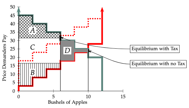
In Figure 8, for the economy presented earlier in Figure 2, we show the tax revenue raised by a 15€ excise tax on profits and its effect on profits of suppliers and demanders. Let the variables \(A\),\(B\),\(C\), and \(D\) denote the areas of the four marked regions in the graph. With no tax, 10 bushels are sold and total profits of demanders and suppliers are given by the sum of the areas, \(A+B+C+D\). With a 15€ excise tax, the solid red supply curve shifts to the dashed red line and in equilibrium, 6 bushels are sold at a price of 31.5. Tax revenue equals the area of the region marked \(C\) which is 6 units wide and 10 units tall. With the tax in place, total profits of buyers are given by the area \(A\), and total profits of sellers are given by the area \(B\). Thus the tax reduces total profits from \(A+B+C+D\) to \(A+B\). Thus the total profits of buyers and sellers must be reduced by \(C+D\) in order to collect a tax revenue of \(C\).
The quantity \(D\) is known as the excess burden of the tax. An excise tax causes excess burden when it excludes some buyers and sellers who could have traded profitably in the absence of a tax. For example, in Figure 8, the tax reduces the number of bushels of apples sold from 10 to 6. The four demanders shut out by the tax include two with Buyer Values of 30 and two with Buyer Values of 25. Also shut out are two suppliers with Seller Costs of 18 and two with Seller Costs of 23. In the absence of a tax, all could make profitable trades, with total profits equalling the area \(D\). But with a 15€ tax, on transactions, none of these can make profitable trades.11
Excess burden is an "excess” in the sense that is the amount by which cost to buyers and sellers of a tax exceeds the amount of revenue raised. In the apple market of our experiment, profits of buyers and sellers depend only on their on sales and are not influenced by the amount of apples sold to others. It is reasonable to assume that nobody cares about how many apples are consumed by other people. But let us consider some of the real-world examples where an excise tax is used. Those who consume gasoline use it to drive on congested roads and subject them to wear and tear. Airline travelers congest airports, which are expensive to maintain. Those who smoke cigarettes impose discomfort on those around them. Excessive alcohol consumption can lead to traffic accidents an other mayhem. Many people believe that marijuana use disturbs social order. These effects are known as externalities. When there are externalities, the total payoffs to individuals may depend not only on what they themselves consume and pay, but may depend on the total consumption of others.
In the example of Figure 8, total consumption is reduced from 10 units to 6 units. Where there are no externalities, this reduction in consumption does not benefit anyone and reduces total profits of those who leave the market by the area \(D\). But if instead of bushels of apples, the commodity were gallons of gasoline, a reduction in the total amount gasoline consumed and hence in congestion on the roads would benefit those who use the roads. Although those who no longer buy or sell gasoline would lose some profit, the resulting gain for those who continue to drive might be greater than the loss \(D\). Thus when there are negative externalities, the reduction in profits to suppliers and demanders might be less than the amount \(C\) of revenue raised.12 This would mean that instead of an "excess burden,” the tax results in an "excess benefit.”
Cigarettes in the United States are taxed both by states and by the federal government. These taxes are collected from cigarette suppliers. State tax rates differ between states and change quite frequently. This makes it possible to estimate the effect of state tax rates on prices paid by cigarette consumers. Studies of the cigarette market (Chiou and Muehlegger 2014; Xiaojin et al. 2015; Evans et al. 1999 ) find that, in the US, changes in state tax rates are almost entirely passed on to consumers in that state.
Gasoline is also subjected to US federal and state excise taxes, which are collected from suppliers. Gasoline tax rates vary from state to state and these rates have changed frequently over time. Studies (Alm, Sennoga and Skidmore 2009; Doyle and Samphantharak 2008) find that, much as with cigarettes, changes in the gasoline tax rate are almost entirely passed on to consumers in the form of higher prices at the pump.
French restaurants pay a value added tax (VAT) for each meal served.13 Changes in the VAT rate charged to restaurants by the French government have enabled economists to estimate the effect of an excise tax on restaurant meals. In 2009, the VAT tax on sit-down restaurant meals in France was reduced from 19.6% to 5.5% of the price of a meal. In 2012 this rate was increased to 7% and 2014 to 10%. A recent study found that only about 25% of the cut in tax rate was passed on to consumers. When the tax rate was increased in 2012 and 2014, prices charged to consumers increased by no more than half of the amount of additional tax.
How do we explain the fact that an excise tax is almost entirely passed on to consumers of cigarettes and gasoline, but not for restaurant diners. The theory we have just learned does the trick. According to competitive supply and demand theory, the fraction of an excise tax that is passed on to consumers is higher, the more responsive (elastic) supply is to price and the less responsive (more inelastic) demand is to price.
Studies find that the demand for cigarettes is quite price inelastic. In Evans et al. (1999), this price elasticity is estimated to be about -0.4 in the short run and -0.7 in the long run.14 Those who are addicted to smoking do not easily give up their habit when the price of cigarettes rises.
What about the supply elasticity? In the short run, the world supply of tobacco is very inelastic. Once the year’s tobacco crop is harvested, the amount available is fixed until the next crop is planted and harvested. But here we are considering the effects of changes in the tax rate charged by a single US state. The number of cigarettes consumed in any state in the US is less than 1% of the total number of cigarettes consumed in the world.15 Even if the total supply of cigarettes is completely inelastic, the elasticity of supply to a state that consumes 1% of the world’s supply is approximately of 100 times as great as the absolute value of the elasticity of demand.16
Studies of the gasoline market find that demand for gasoline is extremely inelastic in the short run, and somewhat more elastic in the long run. A typical estimate (Lin and Prince 2013) has a short run price elasticity of -0.05 and a long run elasticity of -0.25. In the short run, there is little that consumers can do to reduce their gasoline consumption when prices rise. In the longer run, there are more ways to adjust to a price increase. One may buy a more fuel-efficient car, arrange for a work schedule that reduces commuting, or choose to live closer to one’s workplace.
What about the supply elasticity? The incidence of a state-wide tax depends on the elasticity of supply to that state. California, the US state with highest consumption, uses about 2% of world supply. If transportation costs of gasoline could be ignored, this would imply that the supply elasticity for any US state is more than 50 times as large as the absolute value of the demand elasticity.17 Because transportation costs depend on the location of refineries, which can not be changed in the short run, the supply to some states may be somewhat higher in the short run, but we can be confident that, even in the short run, the absolute value of the price elasticity of supply is much greater than that of demand.
In both the cigarette market and the gasoline market, supply is much more responsive to price than is demand. Competitive supply and demand theory predicts that in this case, a state excise tax collected from suppliers will be passed on almost entirely to consumers in the form of higher prices.
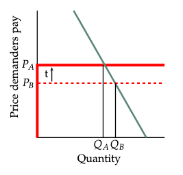
Figure 9 illustrates the effect of an increase in a state excise tax on cigarettes or gasoline. The dashed red line shows the supply curve before a tax increase. We have drawn this supply curve to be nearly horizontal, since supply to a single state is very elastic. If the tax collected from suppliers is increased by the amount \(t\), the supply curve is shifted up by \(t\), since with the tax, when demanders pay \(p\) per unit, suppliers get to keep only \(p-t\). The shifted supply curve is shown as the solid red line. The demand curve is shown by the downward-sloping green line. This line is drawn with a steep slope to represent the fact that demands for cigarettes and gasoline are inelastic with respect to price.
Before the tax increase the supply and demand curves intersected with a price of \(p_B\) and a quantity of \(q_B\). After the tax increase and the supply curve has shifted upwards by \(t\), the new equilibrium has a price of \(P_A\) and quantity \(Q_A\). We see that with the nearly horizontal supply curve and steep demand curve, the price paid by demanders rises by almost the entire amount \(t\) of the tax.
Now let us consider the market for restaurant meals. As you may have guessed, the demand for restaurant meals is much more responsive to price than the demand for cigarettes or gasoline. US Department of Agriculture economists (Okrent and Alston 2012) estimate that the price elasticity of demand for meals in full-service restaurants is about -2, which means that a ten percent increase in the price of meals would result in a 20 percent decrease in demand. The tax changes studied in Benzarti and Carloni (2017) applied to all restaurants in France. While it is possible to ship cigarettes or gasoline to any location in the world, the supply of restaurant meals to French consumers will depend almost entirely on French restaurants who all must pay the same tax rate.
At least in the short run, the supply of meals in French restaurants is likely to be fairly inelastic to price. The number of meals that a restaurant can offer per day is limited by its seating capacity and kitchen facilities. Successful restaurants will be operating at close to full capacity at most meal times, and thus will have limited ability to increase supply when offered a higher price. Therefore it appears that in the market for restaurant meals, demand is more responsive to price than supply. Competitive theory predicts that in this case, less than half of the amount of a tax on French restaurant meals will be passed on to consumers. Figure 10 illustrates the effect of a reduction in an excise tax for restaurant meals. The dashed red line represents the supply curve for a restaurant before a reduction in the tax rate. A reduction in the tax rate per meal by \(t\) shifts the supply curve down by \(t\). The new supply curve is shown as the solid red line. The downward-sloping green line shows the restaurant’s demand curve.
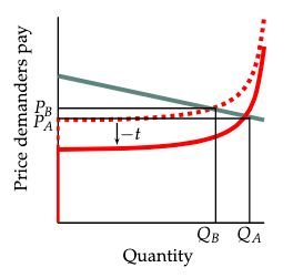
The shape we have chosen for the supply curve can be explained as follows. At prices below the cost of the food and labor that goes into preparing a meal, the restaurant would not be willing to sell any meals. So long as it is operating at less than full capacity, a restaurant is willing to sell meals at any price above the cost of preparing an additional meal. As the number of customers approaches the restaurant’s capacity, in the short run it becomes more expensive, and ultimately impossible, to add more customers. Thus the demand curve has a vertical segment with zero supply at very low prices, a nearly horizontal segment at the cost of handling an extra customer when operating at less than full capacity, and a steeply ascending segment reflecting inelastic supply when the restaurant is operating at full capacity.18 The demand curve is drawn to be highly elastic and to intersect the original supply curve at a point just a bit below full capacity, with price \(P_B\) and quantity \(Q_B\). When the excise tax is reduced by \(t\), the price paid by demanders falls from \(P_B\) to \(P_A\) and the restaurant becomes more crowded with quantity increasing from \(Q_B\) to \(Q_A\). We notice that, just as in the study of the reduction of the VAT on French restaurants (Benzarti and Carloni 2017) the price paid by consumers falls by only about one fourth of the decrease in the tax.
In moving form the old equilibrium to the new, the quantity supplied must increase by just as much as the quantity demanded. With a lower tax rate, this requires a decrease in the price paid by consumers and an increase in the after-tax price received by the restaurant. Since the supply curve is steeper than the demand curve, it must be that the increase in after-tax price for the suppliers is greater in absolute value than the decrease in the price paid by consumers. Thus the price paid by consumers falls by less than half of the reduction in tax.
We have seen the way that the shapes of the supply and demand curves can be used to explain the effect of an excise tax on prices paid by consumers for cigarettes, for gasoline, and for restaurant meals.
Marijuana has recently been legalized in several US states and in Canada. In states where marijuana is legal there is a great variety in state and local tax rates. Which do you think is more responsive to price, demand or supply? Do you think that most of the state or local taxes will be passed on to consumers or will they be absorbed by producers?
The ride-sharing companies, Uber and Lyft, offer a relatively new commodity. A few US states and localities impose a tax on ride-shares with these companies and most do not. Do you think that the fraction of a tax on ride-shares that is passed on to consumers would be greater than or less than the fraction of a tax on marijuana that is passed on?
The United States has both federal and state excise taxes on gasoline. The average total of federal and state taxes is about US $0.52 per gallon (0.12€per liter). The average excise tax on gasoline in European Union countries is about 0.56€per liter ($2.84 per gallon).↩︎
In the US, the average of state and federal excise taxes on cigarettes is about $1.70 (€1.44) per pack. In the European Union, this average is about 3.09€ ($3.64).↩︎
In US states where the sale of marijuana is legal, excise taxes range from 11% to 37% of the retail price.↩︎
The effects of a general sales tax are quite different, because they do not affect the price of the good in question relative to the other taxed goods.↩︎
Social security taxes on labor earnings in the US are an interesting exception. Half of the social security tax is paid by the employer and half by the employee. Real estate transfer taxes are another common exception in many countries. They are imposed on sales of property and it is usually the buyer who pays the tax (in Belgium, Italy or Spain) or is liable for the tax if the seller does not pay it or is exempt (in several states in the US).↩︎
Click these links to see how supply [here] and demand [here] curves are drawn and competitive equilibrium prices and quantities are found. [here]↩︎
If there are a large number of buyers and sellers, each of whom buys or sells a single unit, the "steps” in the demand and supply curves become very small and the curves are well-approximated by smooth curves.↩︎
We measure "steepness” of a curve by the absolute value of its slope.↩︎
In this example, the slopes of the demand curve and supply are constant. If the supply and/or demand curves are not linear, the relevant slopes are the average slopes of these curves over over the range from \(q\) to \(q'\).↩︎
Elasticities of demand and supply are defined as the ratio of the percentage change in quantity demanded or supplied to the percentage change in price as one moves along the demand or supply curve. Economists often prefer to express results in terms of elasticities rather than steepness of demand and supply curves, because elasticities do not change as one changes units of measurement of goods or money, while the steepness depends on the units used. Our proposition states that sharing of the burden is determined by the ratio of the steepness of the demand curve to that of the supply curve. Changes in units of measurement have no effect on this ratio.↩︎
Notice that in the case of a vertical supply curve, an excise tax does not change the number of trades and hence has no excess burden.↩︎
One of our other experiments, the Coal Market Experiment, examines the way in which an excise tax on coal-burning could increase total profits by reducing negative externalities.↩︎
The VAT is an ad valorem tax, meaning that the tax per unit is a fixed fraction of the price charged. The US taxes on cigarettes are per unit tax, where the tax per unit is the same regardless of the price charged. Although this difference has some interesting implications, for the purposes of the current discussion this difference is not essential.↩︎
This means that a 10% increase in the price of cigarettes would reduce demand by about 4% in the short run and 7% in the long run.↩︎
Estimates of cigarette consumption by country can be found at dataverse.scholarsportal.info/dataverse/iccd↩︎
To see this, notice that the supply of cigarettes to a single state is total production, minus total consumption in other regions. If total production does not change, an increase in the pre-tax price of cigarettes in a state that consumes 1% or world supply will reduce the total amount demanded in other states by roughly 100 times as much as it reduces demand in the state with the tax. Thus the absolute value of the price elasticity of supply to the taxed states is about 100 times as great as that of demand from a single state.↩︎
The United States as a whole consumes about 20% of the world’s gasoline. Thus the supply curve of gasoline to the US is much less elastic than that to a single state. We would expect that an increase in the federal gas tax would not be passed on entirely to consumers, but would result in some reduction of the world price of petroleum.↩︎
A more realistic model would account for the fact that there are busy days and less busy days and so a restaurant may be full to capacity on some days and not on others.↩︎